Google Sheets Mastery - Conditional Formatting

There is nothing more satisfying than checking a box and enjoying one thing off your list complete...wait, there is! The whole row strike through or the coloured row! Bold, italicize...<breaths into a paper bag>

I'm back. Sorry about that, I really like using conditional formatting to indicate specific data or to respond to a user. It makes the spreadsheet come alive.

What is conditional formatting? It is the ability to change a cell's (or range, row, column) formatting based on a value.

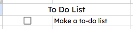
So this:

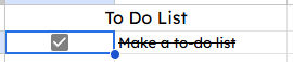
To this:

There are basically two types: Same cell and same and/or other cells.

Want to work along with me? Here is the sample data all typed out.

Same Cell

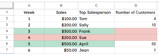
Let's start with this data:

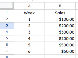
Let's indicate what is greater than $100 in sales.

1. Highlight B2 to B7
2. There are a bunch of ways to get to conditional formatting:
3. Right click, click on "View more cell actions" and then select "Conditional formatting"
4. Click on the font or font background colour and select "Conditional formatting"
5. "Format" -> "Conditional formatting"
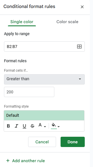
6. In the new window, notice that the range is already added
7. Under "Format cells if..." click on the drop down and select "Greater than".
8. Leave the colour setup alone for now and click "Done"

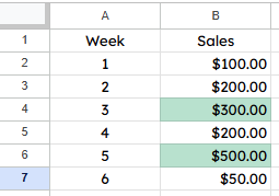
Notice how the $300 and $500 are highlighted in green.

Select B2:B7 again and access the conditional formatting see if you can:

1. Make the numbers less than or equal to $100 show in red.
2. Click on "Color scale" and see if you can get the $50 in red and the $500 in green.

Now that you've had a little practice with the single cell, let's try a row or range.

Same And/Or Other Cells

This is where things get a bit more advanced. We can now specify what we want to change colour based on a value of a cell.

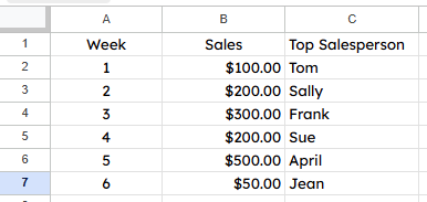
Let's use this example and indicate where the weekly sales are larger than $200:

1. Highlight A2 to C7
2. Activate conditional formatting
3. Leave the range alone
4. At this step you can modify the cells you want to colour but they need to be continuous
5. Click on the drop down under "Format cells if..."
6. Scroll all the way down to "Custom"
7. In the "Value or formula" box enter:
8. =$B2>200
9. $ means that it will only check column B in the range
10. always make sure that the row number (i.e. 2) matches the top row of the range (A2 to C7)

And now we have this:

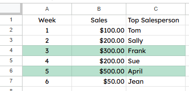
Note: this custom formula can be used on single cells also

One last trick, let's combine a few things to make something really special.

Let's find a way to make this so if the number of customers is blank, it will indicate that:

1. Select A2 to D7
2. Activate conditional formatting
3. Click on the drop down under "Format cells if..." and select "Custom"
4. Enter this into the "Value or formula" box:
5. =$D2=""

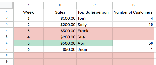
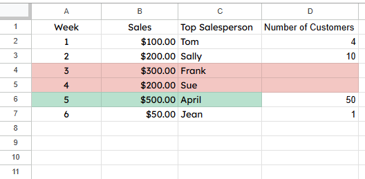
And here are the results:

Well, that is not right. I wanted the row to colour to show that someone forgot to put in the "Number of Customers" which, I think, is more important than Frank and his $300 in sales.

This is where the conditional formatting hierarchy comes in.

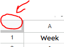
1. Click on the box kitty corner to the A and the 1
2. 
3. Activate conditional formatting
4. Notice that there are two and if you hover your mouse over them, they have a little "grippy" bar to the left:
5. 
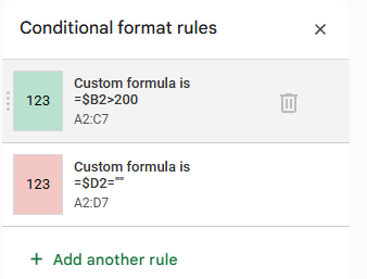
6. Move the top one (i.e. =$B2>200) to the bottom by clicking and dragging on the "grippy" bar
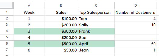
7. Now we get this:
8. 

One last trick...I am always adding in pieces that allow for expansion so what happens if I extend the range all the way down so we can add in further weeks? So, both conditional ranges become "A2:D1000":

That is just p-ugly (pretty ugly!) and not right. Let's go into the conditional formatting and fix this.

1. Click on the box kitty corner to the A and 1.
2. Activate conditional formatting
3. Click on the top conditional format.(i.e. =$D2="")
4. Make sure that the "Apply to range" is set to:
5. A2:D
6. Change the custom equation to:
7. =if(isblank($A2),,$D2="")
8. isblank() -> checks to see if a cell is empty
9. if ->allows the spreadsheet to make a decision
10. in this case, it checks to see if the first cell in the row is blank
11. if it is, do nothing (i.e. nothing between the commas)
12. if it is not blank, do the next thing (i.e. $D="" which checks for an empty customer count)

Note: The $ still must be used or it reverts to a per cell decision and messes it all up.

Well, there is many more items to play with but this should get you started. May your spreadsheets be colourful but meaningful. In the comments below, let me know how you can use conditional formatting to make your job easier.