

At some point, while using a Google App, the thought will occur to you that "there has to be a better way". Sometimes, there is. I had reached the end of the utility of the Google Sheets formulas and needed more from it. This is when I started to dig into Google Scripts.
What is Google Scripts?
It's a strange melding of JavaScript and Google App methods. Use the methods to interact with the App and JavaScript to modify the data.
Google App Script (GScript) is a pretty forgiving programming language (tisking at you C++ and Java!) and here are a few very basic things:
1. Every line must end with an ";"
I've had some instances where I accidentally left them out and nothing went wrong but...most of the time it does something strange.
2. Logger.log() is your best friend
This allows you to display a variable value while the script is running. Code errors are pretty easy to find as the program will tell you there is an error...logic errors are something else entirely hence Logger.log()
3. Debug is also your best friend...maybe even your best man/maid of honour
You can set stop points where the program will display all the values of all the variables at that point. Super handy when you run afoul of an array format.
4. Dot methods can make things really easy
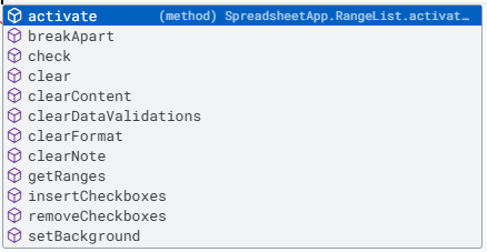
When you use a method (i.e. DocumentApp) and hit a "." after it, the editor provides a list of available options. This is really handy to see if there is an error as the expected options will not appear. The example below will help demonstrate it.
5. Use "//" to make comments...so future you does not cry over past you's opaque programming
Let's make our first Script....using a Macro! Yes, this is completely cheating but will provide your first experience.
Step 1: Open a new spreadsheet (http://sheets.new).
Step 2: Type in "This text will be changed." into cell A1. Copy it to cells A2 through A10.
Step 3: Click back on A1.
Step 4: Go to "Extensions - Macro - Record Macro".
Step 5: Click on "Use relative references".
Step 5: Increase the font size, make it bold, italics, strike through and change the font colour.
Step 6: Click on "Save".
Step 7: Name the macro (i.e. "Text Changer").
Step 8: Enter in "1" in the number box.
Step 9: Click on "Save".

Now we have a nifty little Text Changer macro that can be used in this spreadsheet...and only this spreadsheet.
Click on the cell A2 and then press <CTRL><ALT><SHIFT><1>. Click on the "ok" in the "Authorization required" window. Pick your account and then "Allow".
What does this do? It is a security feature of Google and makes sure it can run this script on your account in this document.
...and nothing happened! That was just to set security. It will now run every time after. Give it another try by pressing <CTRL><ALT><SHIFT><1>!
Like magi, it changed the text in the new cell...because we selected "relative referencing" so it uses the current cell selected instead of always changing A1 which would be a really boring script.
I can already hear you saying..."but I thought this was programming?!?!". Let's lift the curtain on that.
Step 1: Go to "Extensions - App Script". This is where all the programming lives.
Step 2: Bask in the glory of a "simple" script flawlessly programmed!
Notice the setup:
function TextChanger() { //starts with the function
var spreadsheet = SpreadsheetApp.getActive(); //tells the script it will be using this spreadsheet
spreadsheet.getActiveRangeList().setFontSize(13) //changes all the attributes
.setFontWeight('bold')
.setFontStyle('italic')
.setFontLine('line-through')
.setFontColor('#0000ff'); //notice the ";" which indicates the end of the changes for the spreadsheet
}; //this is how it completes the function
Let's play a little. Put your cursor at the end of the line of ".setFontStyle('Italic')". Press enter then type ".". Notice all the options...these are all the "methods" or all the things you can add or change about the cell selected.
Hmm...take a look back over the code above. Notice how it says ".getActiveRangeList()". What could that mean? Close down the Script window and click on "Leave" as we do not want to save the latest changes.
Head back to the spreadsheet and select cells A3 to A10. Activate the macro again and...voila! It applies the changes to all the cells you have selected (hence Active Range List!).
Obviously, this is just the start of the journey. Let me know in the comments what you think or what you would like to learn next. The options are endless!
Comments ()