College Savings Planner Excel

College Savings Planner Excel — Every college account in one plan: 529s, brokerage, ESA and cash funds, with percent funded and months to goal.

Built for anyone who wants the whole picture on one page: what the goal is, what is actually there, and which line is quietly falling behind — without accounting software or a subscription app. If one line is underfunded, this workbook shows it while there is still time to fix it.

WHAT'S INCLUDED (6 sheets):

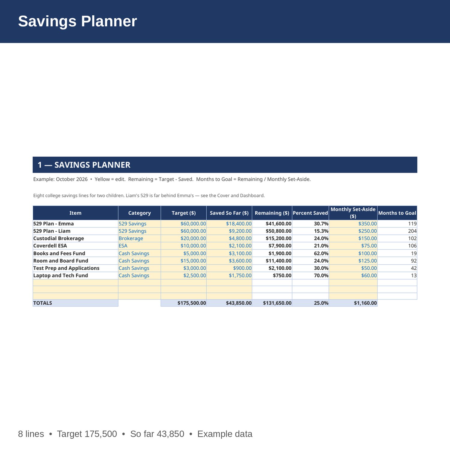
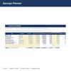
- Savings Planner — Every college account: target, saved so far, remaining, percent saved, monthly contribution, and months to goal — by formula except the yellow inputs.

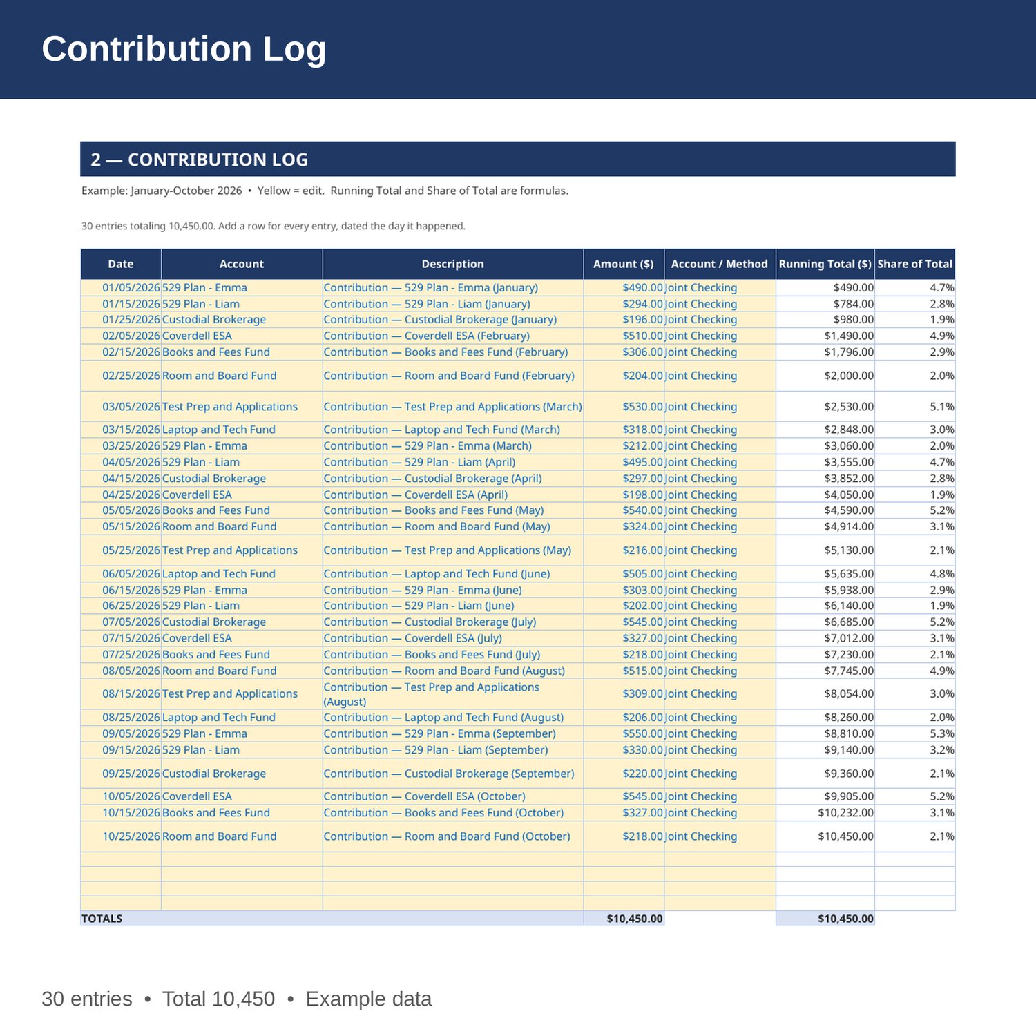
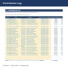
- Contribution Log — Every contribution January-October: date, account, description, amount, and source account, with running total and share of total by formula.

- Monthly Plan — Month by month: planned contributions, actual contributions from the log by formula, the difference, and cumulative planned vs actual.

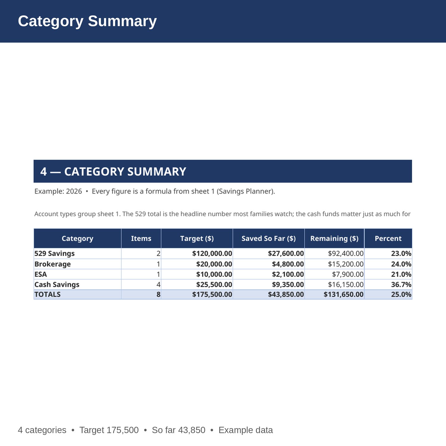
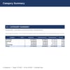
- Category Summary — Accounts grouped by type (529, brokerage, ESA, cash): counts, targets, saved, remaining, and percent saved — all by formula.

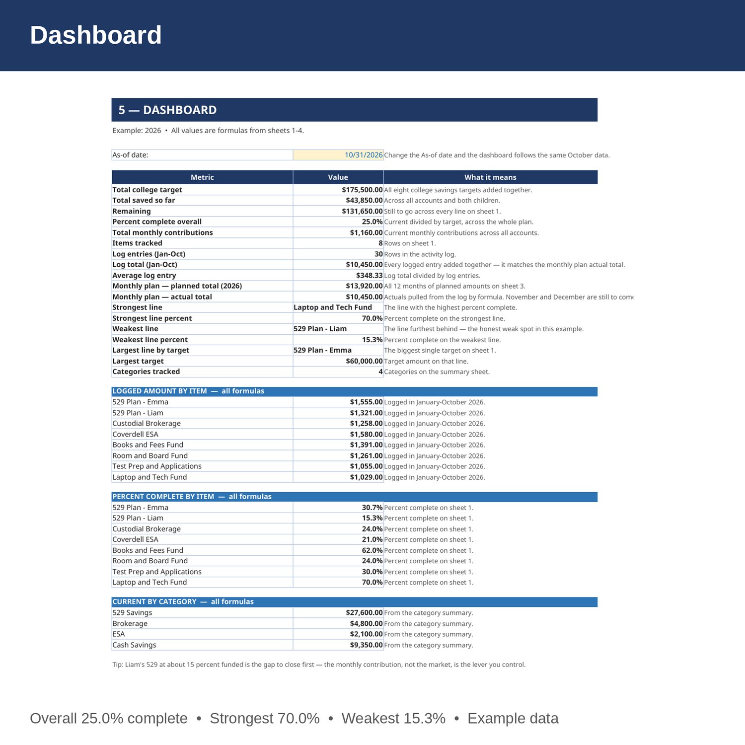
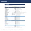
- Dashboard — Total college target, total saved, remaining, percent funded, monthly contributions, and the strongest and weakest accounts.

- Cover and How to Use — start here. Yellow cells are the only ones you edit.

EXAMPLE DATA (2026 — replace with your own numbers):

- Target 175,500; current 43,850; remaining 131,650; 25.0 percent complete overall.

- 30 logged entries (January-October 2026) totaling 10,450; monthly plan planned 13,920 for 2026 against actual 10,450 so far.

- Strongest line: Laptop and Tech Fund at 70.0 percent. Weakest line: 529 Plan - Liam at 15.3 percent. Largest line: 529 Plan - Emma at 60,000.

HOW IT WORKS:

1. Download the Excel file instantly after purchase.

2. On sheet 1, enter each account's target, balance saved so far, and monthly contribution. Remaining, percent, and months fill in by formula.

3. On sheet 2, add a row per contribution: date, account (spelled exactly as on sheet 1), amount, and source.

4. On sheet 3, set planned contributions per month. Actuals land by formula from the log.

5. Sheets 4 and 5 summarize everything by formula. Check them monthly.

HOW THE NUMBERS WORK:

Remaining is the target minus the current amount. Percent is the current amount divided by the target. Months figures divide the remaining amount by the monthly amount, rounded up. Monthly actuals are the sum of log entries in that month. Category totals group sheet 1 by its category column. Nothing in the example assumes investment growth or interest unless a sheet says so in plain words.

PLEASE NOTE:

- Instant digital download. No physical item ships.

- Works in Microsoft Excel and Google Sheets (upload to Google Drive to open in Sheets).

- Example data is included so you can see how it works. Replace the yellow cells with your own numbers — yellow cells are the only ones you edit.

- This is a bookkeeping tool, not tax, legal, or CPA advice.

- Built by an accountant: B.S. Accountancy, ASU W. P. Carey, with revenue-reconciliation experience at Marriott and audit work at PwC.