

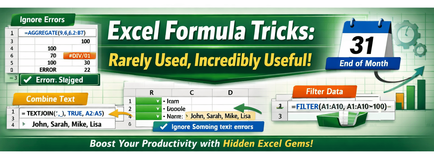
AGGREGATE — Skip Errors and Get Accurate Totals
Why Use It
When your data has errors like #DIV/0!, normal formulas fail. AGGREGATE ignores those errors automatically.
Steps
- Select the cell where you want the total.
- Type: =AGGREGATE(9,6,B2:B7)
- Press Enter — Excel calculates the sum while skipping error cells.
Legend:
- Green arrow → Formula cell
- Red arrow → Error cells ignored
- Blue arrow → Final total
Result: You’ll see a clean total even if some entries are broken.
TEXTJOIN — Combine Text Easily
Why Use It
Perfect for merging names, departments, or codes into one neat line.
Steps
- Select a cell for the combined text.
- Type: =TEXTJOIN(", ", TRUE, A2:A5)
- Press Enter — Excel joins all names with commas.
Legend:
- Yellow arrow → Source cells (A2:A5)
- Green arrow → Formula cell
- Blue arrow → Combined result
Result: “John, Sarah, Mike, Lisa” — clean and ready for reports.
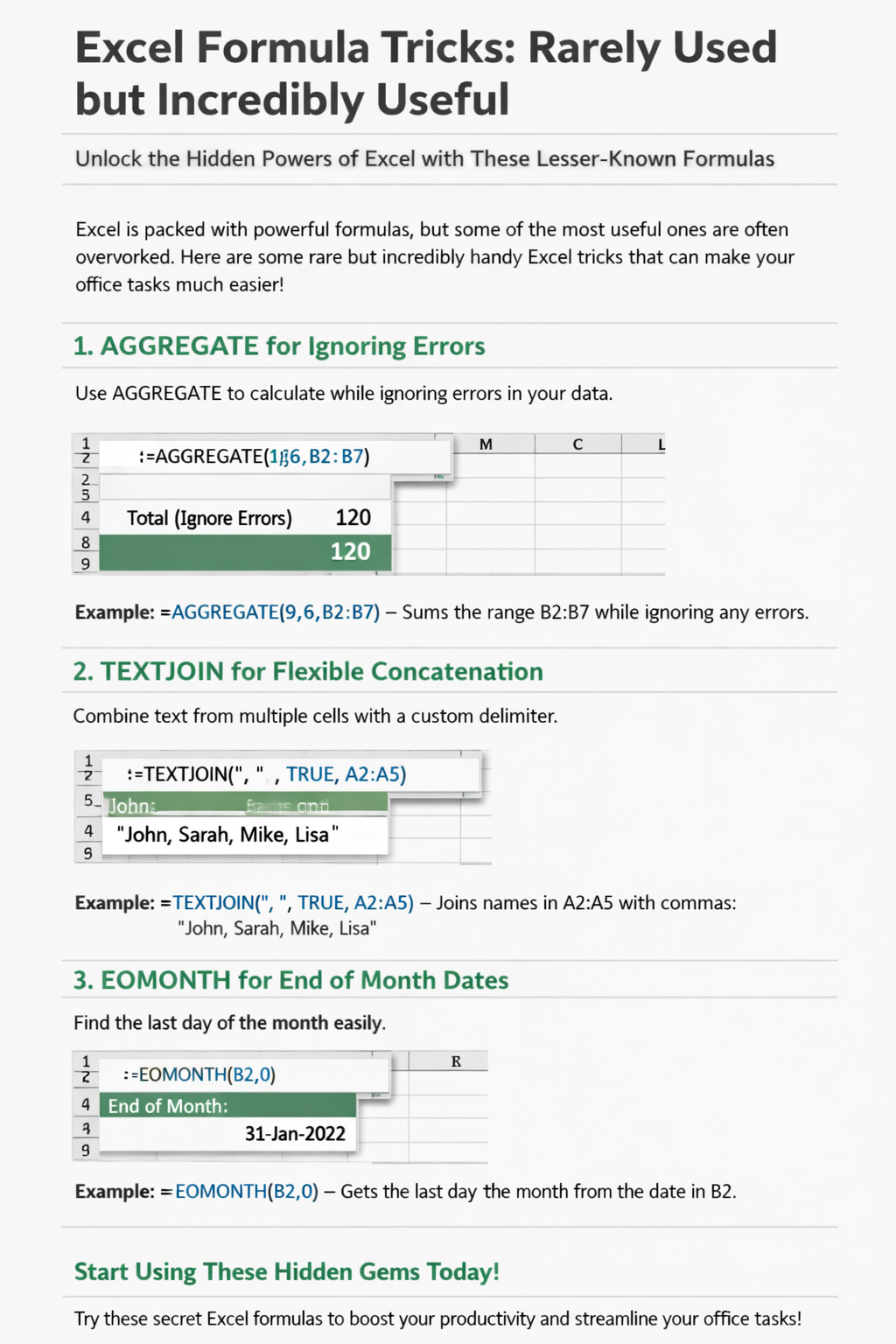
EOMONTH — Find the Last Day of Any Month
Why Use It
Ideal for payroll, billing, or scheduling tasks.
Steps
- Select a cell for the end date.
- Type: =EOMONTH(B2,0)
- Press Enter — Excel returns the month’s last day.
Legend:
- Orange arrow → Date input (B2)
- Green arrow → Formula cell
- Blue arrow → Result (last day of month)
Result: “31‑Jan‑2022” — automatically adjusts for any month.
Bonus Tips
- Use UNIQUE to remove duplicates instantly.
- Try FILTER for dynamic reports.
- Clean messy text with TEXTSPLIT.
TEXTSPLIT — Split Cell Values by Delimiter
Why Use It
When you have data like "Juan Dela Cruz, HR, Manila" in one cell, TEXTSPLIT can separate each part automatically.
Steps
- Select a cell where you want the split results to appear.
- Type: =TEXTSPLIT(A2,",")
- Press Enter — Excel divides the text into columns or rows based on the comma.
Legend:
- Green arrow → Formula cell
- Yellow arrow → Original text cell
- Blue arrow → Separated results
💡 Result:

Perfect for cleaning imported CSV data or employee lists.
TEXT — Display Only 3 Letters of a Month
Why Use It
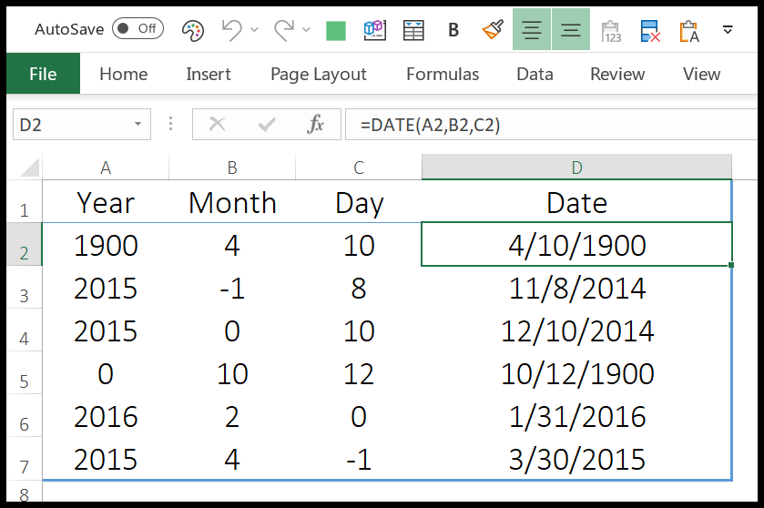
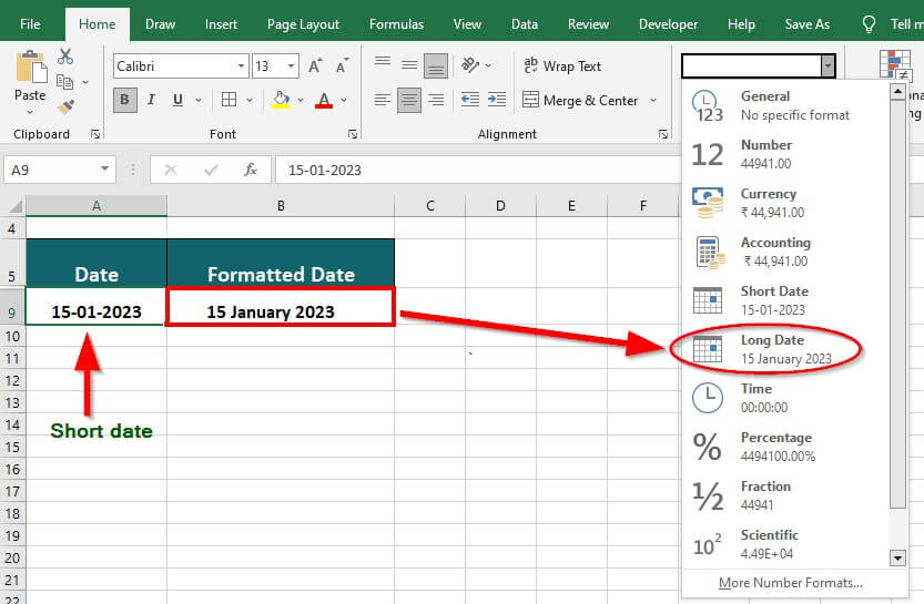
If your date shows “January 2026,” you can shorten it to “Jan” automatically — great for compact reports.
Steps
- Select a cell with a full date (e.g., B2 = 15-Jan-2026).
- Type: =TEXT(B2,"mmm")
- Press Enter — Excel converts the month to its three-letter abbreviation.
Legend:
- Green arrow → Formula cell
- Orange arrow → Original date cell
- Blue arrow → Result (month abbreviation)
Result: Jan — automatically updates if the date changes.
SUMMARY:
AGGREGATE for error-free totals
TEXTJOIN for merging text
EOMONTH for end-of-month dates
TEXTSPLIT for delimiter-based splitting
TEXT for month abbreviations
If you found this blog helpful, share it with your fellow educators, and let’s keep the conversation going on the future of digital schooling in the Philippines!
Ed is the founder of DigiScape Toolbox, creating digital tools that help teachers automate tasks and improve efficiency.